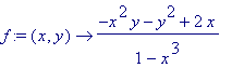
>   

restart:with(DEtools):with(plots):f:=(x,y)->(-(x^2)*y-y^2+2*x)/(1-x^3);eq:= D(y)(x)=f(x,y(x));
yo:=1;sol1:=dsolve({eq,y(0)=yo},y(x));y1:=normal(subs(sol1,y(x)));

>   

z:=proc(n,xo,yo,f,A)
          local i,x,h;

        option remember;
  
 for i from 0 to n-1 do A[i]:=unassign(`A[i]`); od;
     h:=xo/n;A[0]:=yo;
     for i from 0 to (n-1)
        do  x:= i*h;A[i+1]:=A[i]+h*f(x,A[i]);od;
end:          

>   

with(plots):
xo:=0.99:A[0]:=yo:n:=10:z(n,xo,yo,f,A):
a1:=evalf(min(seq(A[i],i=0..n)));a2:=evalf(max(seq(A[i],i=0..n)));
:eval(A):
n:=20:z(n,xo,yo,f,B):b1:=evalf(min(seq(B[i],i=0..n)));b2:=evalf(max(seq(B[i],i=0..n)));
n:=100:z(n,xo,yo,f,C):
c1:=evalf(min(seq(C[i],i=0..n)));c2:=evalf(max(seq(C[i],i=0..n)));

>   

with(plottools):seq_opt:=x=-0.05..xo,y=min(a1,b1,c1,a2,b2,c2)..max(a1,b1,c1,a2,b2,c2)+0.05,color=black:
Z1:=plot([seq([i*xo/10,A[i]],i=0..10)],seq_opt,linestyle=1):
Z2:=plot([seq([i*xo/20,B[i]],i=0..20)],seq_opt,linestyle=2):
Z3:=plot([seq([i*xo/100,C[i]],i=0..100)],seq_opt,linestyle=3):
Y1:=plot(y1,x=0..xo,color=red):l:=disk([0,yo],0.002,color=red):
display({Z1,Z2,Z3,Y1,l});

>   

restart:with(plots):with(DEtools):with(plottools):

>   

z:=proc(n1,n2,n3,xo,yo,f)
          local i,x,h,a1,a2,A,B,C,seq_opt,Z1,Z2,Z3,Y1,eq,sol1,y1,l;

  initialisation des tables A,B,C contenant les ordonnées des points des lignes polygonales   
 for i from 0 to n1-1 do A[i]:=unassign(`A[i]`);od;
 for i from 0 to n2-1 do B[i]:=unassign(`B[i]`);od:
 for i from 0 to n3-1 do C[i]:=unassign(`C[i]`);od:
résolution de l'équation différentielle y'=f(x,y)
eq:= D(y)(x)=f(x,y(x));
sol1:=dsolve({eq,y(0)=yo},y(x));y1:=unapply(rhs(sol1),x);
Détermination des tables A,B,C  
     h:=xo/n1;A[0]:=yo;
     for i from 0 to (n1-1)
        do  x:= i*h;A[i+1]:=A[i]+h*f(x,A[i]);od;
  
     h:=xo/n2;B[0]:=yo;
     for i from 0 to (n2-1)
        do  x:= i*h;B[i+1]:=B[i]+h*f(x,B[i]);od;

     h:=xo/n3;C[0]:=yo;
     for i from 0 to (n3-1)
        do  x:= i*h;C[i+1]:=C[i]+h*f(x,C[i]);od;
Détermination des extremas des ordonnées
a1:=evalf(min(seq(A[i],i=0..n1),seq(B[i],i=0..n2),seq(C[i],i=0..n3)));
a2:=evalf(max(seq(A[i],i=0..n1),seq(B[i],i=0..n2),seq(C[i],i=0..n3)));
seq_opt:=0..xo,y=a1..a2,color=black:
Z1:=plot([seq([i*xo/n1,A[i]],i=0..n1)],seq_opt,linestyle=2):
Z2:=plot([seq([i*xo/n2,B[i]],i=0..n2)],seq_opt,linestyle=1):
Z3:=plot([seq([i*xo/n3,C[i]],i=0..n3)],seq_opt,linestyle=3):
Y1:=plot(y1,seq_opt,color=red):

l:=disk([0,yo],0.002,color=blue):
display({Z1,Z2,Z3,Y1,l});
end:

>   

>   

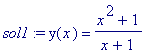
f:=(x,y)->(-(x^2)*y-y^2+2*x)/(1-x^3);eq:= D(y)(x)=f(x,y(x));
xo:=0.99:yo:=1;
z(10,20,100,xo,yo,f);